Winch Model in Matlab
The model of the winch can be implemented in Matlab instead of Julia. The rest of the simulation stays in Julia: the kite and tether model (KiteModels.jl), the winch controller (WinchControllers.jl), the flight path controller and the state machine SystemStateControl. The Matlab winch is driven by SystemStateControl through the Julia winch controller for the full power cycle: parking, power production, reel-in and depower.
The Matlab function examples/matlab/async_machine_step.m implements the same model as the AsyncMachine of WinchModels.jl: an asynchronous machine with gearbox, drum, friction and brake. It is a starting point for your own Matlab winch models.
Requirements
- Matlab R2020b or newer, with a license that allows starting the Matlab engine. Matlab Coder is not needed. Octave is not supported.
- On Linux,
csh(the Matlab engine is started with it). - WinchModels.jl 0.3.13 and KiteModels.jl 0.13.2 or newer, which support the
MatlabMachine;Pkg.instantiate()installs them (see Setup).
Setup
The Matlab examples have their own environment, examples/matlab, because MATLAB.jl cannot be installed without Matlab. In a Julia session started in the root folder of KiteControllers.jl:
using Pkg
Pkg.activate("examples/matlab")
ENV["MATLAB_ROOT"] = "/usr/local/MATLAB/R2021a"   # only if the wrong Matlab is found
Pkg.instantiate()
Pkg.build("MATLAB")
Packages in the system image cannot be replaced by other versions. To work on development versions of WinchModels.jl or KiteModels.jl, start Julia without the system image with bin/run_julia --nosysimage.
Usage
Autopilot with the Matlab winch
Choose autopilot_matlab in the menu of the examples (menu()), or run:
include("examples/autopilot_matlab.jl")This runs autopilot.jl with the Matlab winch model instead of the winch model of the selected project. If the active environment is not examples/matlab, for example when started from the menu, the script starts a new Julia process for it, without system image, and waits until the window is closed.
Selecting the Matlab winch in the settings
In your own scripts, set the winch model in the settings file of the project:
winch_model: "MatlabMachine" # or AsyncMachine or TorqueControlledMachineand load MATLAB.jl and add the folder of the Matlab function to the Matlab path before the first time step. Start the Matlab engine before Pkg or Downloads are loaded, which KiteUtils.jl and the packages that use it do: with Matlab R2025a, starting the engine later crashes Julia (segmentation fault), probably because Julia and Matlab use different versions of libcurl. mat"..." starts the engine:
using MATLAB
mat"addpath('examples/matlab')"
using KiteModels
KPS3 and KPS4 then create a MatlabMachine. An unknown value of winch_model stops with an error.
How it works
The acceleration of the winch is calculated in the residual of the DAE solver, which evaluates it many times per time step. A call of Matlab costs about a millisecond, so Matlab is called only once per time step, in update_winch_state! of WinchModels.jl:
- Julia passes the reel-out speed and the tether force at the start of the time step, the set speed of the winch controller and the state of the brake and of the rate limiter of the set speed.
async_machine_step.mupdates the brake and the rate limited set speed and returns the acceleration and its partial derivatives with respect to speed and force.- Within the time step, the residual uses the first order expansion
acc0 + dacc_dv*(speed - speed0) + dacc_dF*(force - force0), evaluated in Julia.
Linearization within the time step
Within one time step, the set speed, the state of the brake and the parameters are constant, so the acceleration of the winch is a function of the reel-out speed v and the tether force F only:
acc = f(v, F)At the start of each time step, Matlab evaluates this function once at the current point (v0, F0) and returns its value and its two slopes:
acc0    = f(v0, F0)
dacc_dv = ∂f/∂v (v0, F0)
dacc_dF = ∂f/∂F (v0, F0)
During the time step, the DAE solver needs the acceleration many times, at slightly different values of v and F. Instead of calling Matlab, it uses the tangent plane through this point, the first two terms of the Taylor series (first order expansion):
acc ≈ acc0 + dacc_dv * (v - v0) + dacc_dF * (F - F0)The error of this approximation depends on how curved f is:
- In the force there is no error: the force enters the torque balance linearly, so
dacc_dFis constant. - In the speed there is an error: the motor torque depends on the slip
δ = ω_sync - ωasδ / (R² + L²δ²), and the Coulomb friction is a smooth sign function of the speed. The error grows approximately with½ ∂²f/∂v² (v - v0)², quadratically with the change of the speed within the time step and with the curvature of the torque-slip curve. - With the brake engaged there is no error: the acceleration is
brake_acc * v, which is linear.
The error is therefore largest when the speed changes a lot within one time step in a strongly curved part of the torque-slip curve, for example at the transitions between reel-out and reel-in. Over full power cycles the effect is small, see Accuracy. If more accuracy were needed, Matlab could also return the second derivative ∂²f/∂v², and Julia would add the quadratic term; this still needs only one call of Matlab per time step.
Calling Matlab
The parameters (gear ratio, drum radius, inertia, friction, maximal acceleration, motor data) are sent to Matlab once, before the first time step. The Matlab engine is called by the package extension WinchModelsMATLABExt, which is loaded by using MATLAB: one evaluation per time step with the inputs as text, without the exception check of MATLAB.jl, and one read of the result vector. Errors in Matlab are reported as Julia errors.
Accuracy
examples/matlab/compare_full_cycle.jl flies the power cycles of autopilot.jl, without viewer and turbulence, with the Julia AsyncMachine and with the MatlabMachine, for 460 s:
| project | energy, Julia | energy, Matlab | difference |
|---|---|---|---|
| hydra10_951 | 654.2 Wh | 654.3 Wh | 0.014 % |
| hydra20_426 | 752.3 Wh | 752.4 Wh | 0.018 % |
| hydra20_600 | 1759.4 Wh | 1760.2 Wh | 0.044 % |
| hydra20_920 | 1555.1 Wh | 1557.8 Wh | 0.177 % |
Mean and maximal tether force differ by at most 0.13 %. The difference comes from the linearization within the time step. examples/matlab/test_async_machine_step.jl checks that the Matlab function itself agrees with the Julia model to 1e-12.
Speed
One time step with the Matlab winch takes about 1.5 ms (median) and 2.2 ms (99th percentile), measured with Matlab R2021a on Linux, compared to less than 0.1 ms with the Julia winch model. The simulation is real-time capable up to a time-lapse factor of about 18 (2.8 ms per time step of 50 ms); 24 is too fast. The 3D viewer of autopilot.jl needs additional time.
The speed of the Matlab engine depends on the computer and the Matlab version. On a laptop with Matlab R2025a, one time step took about 4.3 ms (median) and 7 ms (99th percentile), and a call of the engine was about 2.5 times slower than with R2021a on the first computer. There, the simulation is real-time capable up to a time-lapse factor of about 6; with 12 it missed every deadline. Choose the time-lapse factor in the menu of autopilot.jl accordingly. examples/matlab/bench_engine.jl measures the cost of different ways of calling Matlab.
Your own Matlab winch model
Replace the body of async_machine_step.m and keep its interface:
async_machine_step(p)    % store the parameter struct p
y = async_machine_step(x)
% x = [speed, force, set_speed, use_brake, brake, last_set_speed]
% y = [acc0, dacc_dv, dacc_dF, brake, last_set_speed]
set_speed is NaN if there is no set speed. The model is called once per time step, so it may keep its own state in persistent variables, but the brake and the rate limited set speed must be returned, because KiteModels saves and restores them. The partial derivatives must describe the acceleration within the time step well; the accuracy of the simulation depends on them.
Testing the model in Matlab
examples/matlab/winch_example.m runs the winch model in Matlab alone, without Julia. Use it to try out changes of the model before running it in the full simulation. In Matlab, in the folder examples/matlab:
winch_exampleThe script sets the parameters as Julia loads them for system.yaml and simulates the winch for 20 s with a time step of 50 ms. The set speed follows a profile, and the tether force is prescribed for each part:
| time | set speed | tether force | |
|---|---|---|---|
| 0 to 2 s | 0 | 1000 N | brake engaged |
| 2 to 8 s | 4 m/s | 3000 N | reel-out |
| 8 to 14 s | -6 m/s | 800 N | reel-in |
| 14 to 20 s | 0 | 1000 N | brake engaged again |
As in the Julia simulation, async_machine_step is called once per time step. The speed is integrated with the linearized implicit Euler method, using the partial derivative dacc_dv: v(t+dt) = v(t) + dt * acc0 / (1 - dt * dacc_dv). An explicit Euler step would be unstable, because the torque-slip curve of the machine is steep.
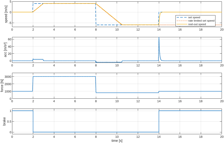
The reel-out speed follows the set speed with the maximal acceleration of 4 m/s², and differs from it by at most 0.063 m/s while reeling out. At t = 14 s the brake stops the winch within about 0.3 s. While the brake is engaged, the rate limited set speed keeps its last value.
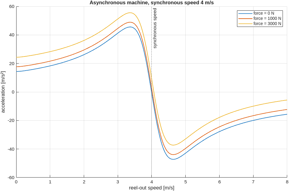
A second figure shows the acceleration as a function of the reel-out speed for a synchronous speed of 4 m/s, the torque-slip curve of the asynchronous machine. Near the synchronous speed the curve is steep and almost linear, further away it is strongly curved: there, the linearization within the time step is least accurate.
Limitations
- Only the asynchronous machine is available in Matlab, not the
TorqueControlledMachine. - Matlab holds the parameters of one
MatlabMachineat a time; they are sent again when anotherMatlabMachineis used. Change the parameters of aMatlabMachinebefore its first time step. - The Matlab engine adds about 1.5 ms per time step, see Speed.